the Creative Commons Attribution 4.0 License.
the Creative Commons Attribution 4.0 License.
 | 05 Jun 2018
Country-level assessment of future risk of water scarcity in Europe
Ana Iglesias
Alfredo Granados
A methodology for regional assessment of current and future water availability in Europe is presented in this study. The methodology is based on a proposed indicator of risk of water scarcity based on the projections of runoff and water availability for European countries. The risk of water scarcity is the combined result of hydrological processes, which determine streamflow in natural conditions, and human intervention, which determines water management using the available hydraulic infrastructure and establishes water supply conditions through operating rules. Model results show that changes in runoff and availability obtained for individual GCM projections can be large and even contradictory. These heterogeneous results are summarized in the water scarcity risk index, a global value that accounts for the results obtained with the ensemble of model results and emission scenarios. The countries at larger risk are (in this order) Spain, Portugal, Macedonia, Greece, Bulgaria, Albania, France and Italy. They are mostly Mediterranean countries already exposed to significant water scarcity problems. There are countries, like Slovakia, Ireland, Belgium, Luxembourg, Croatia and Romania, with mild risk. Northern Arctic countries, like Sweden, Finland, Norway and Russia, show a robust however mild increase in water availability.


There is a growing concern about the possible impacts of climate change on water resources availability (Arnell, 2004). Regional assessments are an important tool to provide decision makers with a global picture of future situations according to hypothesized future socio-economic pathways (Alcamo et al., 2000). Decision makers require projections several decades ahead, but they are faced with very large uncertainties. There is a multiplicity of future scenarios of physical variables deriving from different emission scenarios and uncertainties inherent to the modelling tools used in the analysis. Other variables are even more uncertain due to the complexity of the socioeconomic system.
Many regional studies have been carried out to obtain projections of water availability. Arnell (1999) presented one of the first regional studies for Europe. The most up to date summary is the last Assessment Report of the Intergovernmental Panel on Climate Change (IPCC) (IPCC, 2014). Most of these studies assimilate global climate model (GCM) results into water resources impact-assessment models, either by downscaling climate model results to a finer scale (Fowler et al., 2007; Fronzek and Carter, 2007) or by developing macroscale hydrological models (Sperna Weiland et al., 2012, van Beek and Bierkens, 2009). Assessment of impacts on water resources requires also analysis of the projected evolution of water demands (Döll, 2002; Alcamo et al., 2007; Wisser et al., 2008) and simulation of water management practices (Gleick, 2003; Alcamo et al., 2003a). In Europe, water resources systems are highly developed and have achieved a profound transformation of the natural characteristics of water flow to adapt to variability and uncertainty. The WaterGAP model (Alcamo et al., 2003b) is a good example of integration of diverse modelling tools to account for the human intervention on the natural system under climate change scenarios.
In this paper we present a methodology to assist decision makers in dealing with uncertainties in projections of water resources scenarios under climate change. The methodology is based on a proposed water scarcity risk index, a global value that accounts for the results obtained with the ensemble of model results and emission scenarios.
The methodology is applied to conduct a country-level assessment of risk of water scarcity in Europe. We first present the methodology to obtain projected changes of runoff and water availability. Projected changes in runoff were inferred from the results of the PCR-GLOBWB hydrologic model and projected changes in water availability were estimated with the Water Availability and Adaptation Policy Analysis (WAAPA) model. We later introduce the methodology to compute the water scarcity risk index and apply it to Europe.
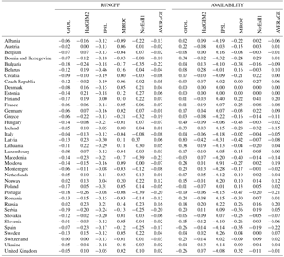
Table 1Country estimates of changes in average runoff and surface water availability in the long term period (2060–2099) with respect to the control period (1960–1999) under emission scenario RCP4.5. Results show the five GCM 40 forcing models considered and the average value.
In this section we introduce the model developed for the river basins of Europe and the estimation of runoff and water availability projections. A detailed presentation of the model can be found in Garrote et al. (2015a).
2.1 Model configuration
Model topology was taken from the “Hydro1k” data set (EROS, 2008). We identified 1260 subbasins of average size around 5000 km2. The reservoir storage volume available for regulation in every subbasin was obtained from the ICOLD World Register of Dams (ICOLD, 2004). Dams in the register with more than 5 hm3 of storage capacity were georeferenced and linked to the corresponding storage capacity and flooded area. It was assumed that all reservoir storage available in a given subbasin was concentrated in a single equivalent reservoir located at the basin outlet. Environmental flows were computed through hydrologic methods. Monthly minimum required environmental flow was defined as the 10 % quantile in the distribution of naturalized monthly flows.
2.2 Climate scenarios
The climate scenarios were provided by five different climate model combinations that were used to force the PCR-GLOBWB model: GFDL-ESM2NM, HadGEM2-ES, IPSL-CM5A-LR, MIROC-ESM-CHEM and NorESM1-M. The models were run from 1960 to 2099 under two Representative Concentration Pathways emission scenarios: “RCP4.5” and “RCP8.5”. Three time slices were considered for analysis: “Control (CTL)” (1960–1999), “Short term (ST)” (2020–2059) and “Long term (LT)” (2060–2099).
2.3 Projections of runoff
Naturalized streamflow was obtained from the results of the application of the PCR-GLOBWB model (van Beek and Bierkens, 2009) to the Inter-Sectoral Impact Model Intercomparison Project (Warszawski et al., 2014). The PCR-GLOBWB model was run for the entire globe at 0.5∘ resolution using forcing from the five GCMs under control conditions and climate change. These results are available for downloading from the CORDEX data portal.
The runoff provided from the PCR-GLOBWB models was interpolated on a finer grid to obtain monthly time series of streamflow in each basin. An example of the average runoff obtained with one of the forcing GCMs (GFDL) for the control period is presented in Fig. 1.
Figure 1 also presents the spatial distribution of relative changes in runoff for the long term period under emission scenario RCP4.5 compared to the control period for the GFDL climate forcing.
Relative changes are calculated following Eq. (1):
Where RCTL is the average runoff for the control period and RRCP is the average runoff for the future period.
Average runoff values in the control period were compared to the global composite runoff field of the University of New Hampshire Global Runoff Data Centre (UNH/GRDC), which combines observed river discharges with a water balance model (Fekete et al., 2002). The results are shown in Fig. 2. All climate forcing models produced similar results, with strong positive bias. For this reason, PCR-GLOBWB simulations were corrected for the bias observed in the control period.
2.4 Projections of water availability
Water availability is estimated for every subbasin through the WAAPA model (Garrote et al., 2015b). The objective of the WAAPA model is to simulate the operation of a water resources system to maximize water availability.
In this study WAAPA model was used to estimate maximum potential water availability in the European river network applying gross volume reliability as performance criterion. The simulation consists on estimating the maximum demand that can be supplied at a given point of the river network considering the upstream basin: all the series of streamflow and available reservoir storage in all upstream nodes. All upstream reservoirs are jointly managed to satisfy the total demand located at the basin outlet. The demand is satisfied if it can be met with a given reliability criterion. The criterion used in the analysis was 98 % reliability in volume.
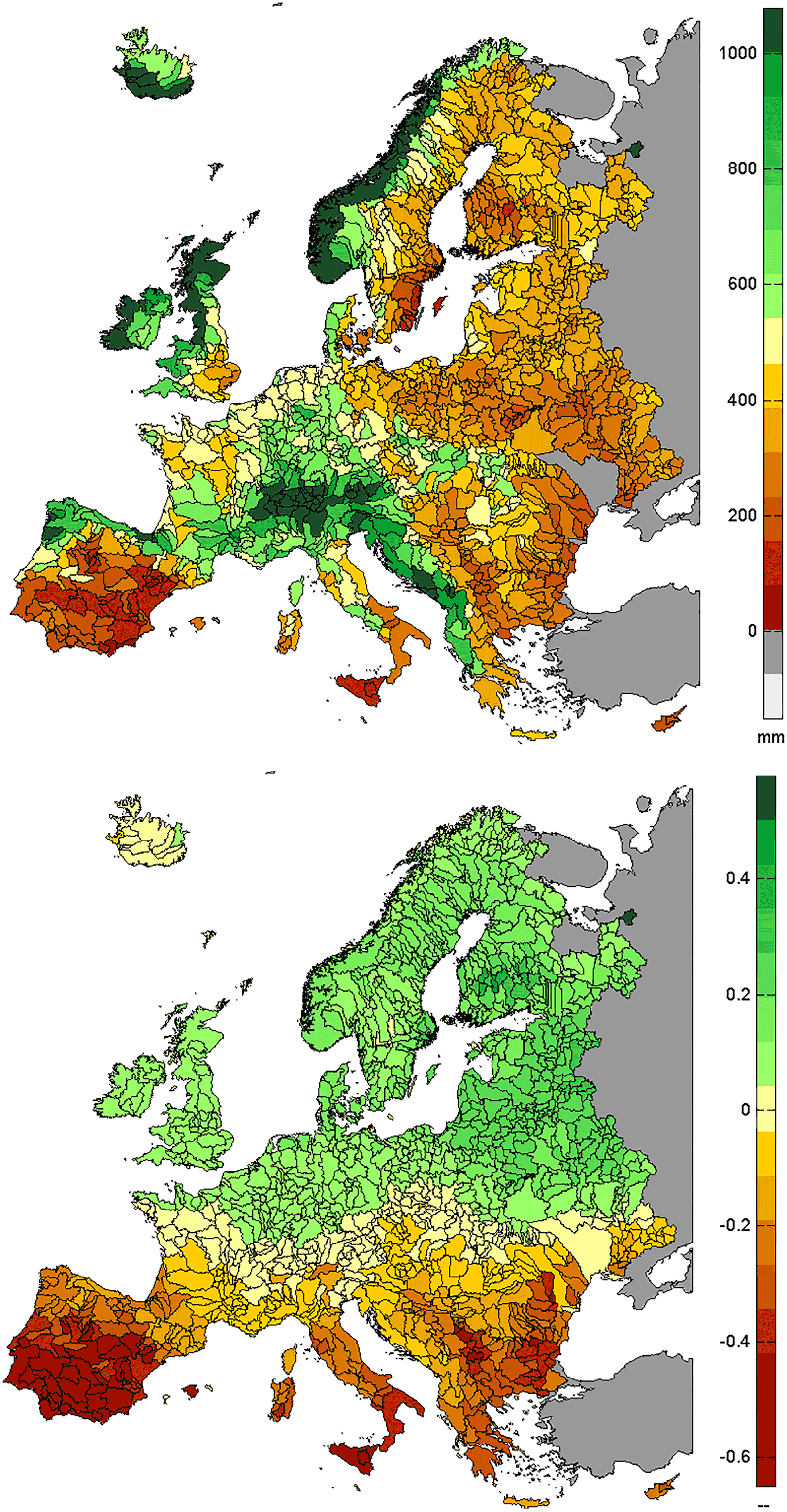
Figure 1Subbasin average runoff (in mm) in the control period (1960–1999) and relative changes in the long term period (2060–2099) under emission scenario RCP4.5 according to PCR-GLOBWB model forced with GFDL climate data.
Basic components of WAAPA are inflows, reservoirs and demands. These components are linked to nodes of the river network. WAAPA allows the simulation of reservoir operation and the computation of supply to demands from a system of reservoirs accounting for ecological flows and evaporation losses. From the time series of supply volumes, supply reliability can be computed according to different criteria. Water availability is linked to the point in the river network where it is calculated.
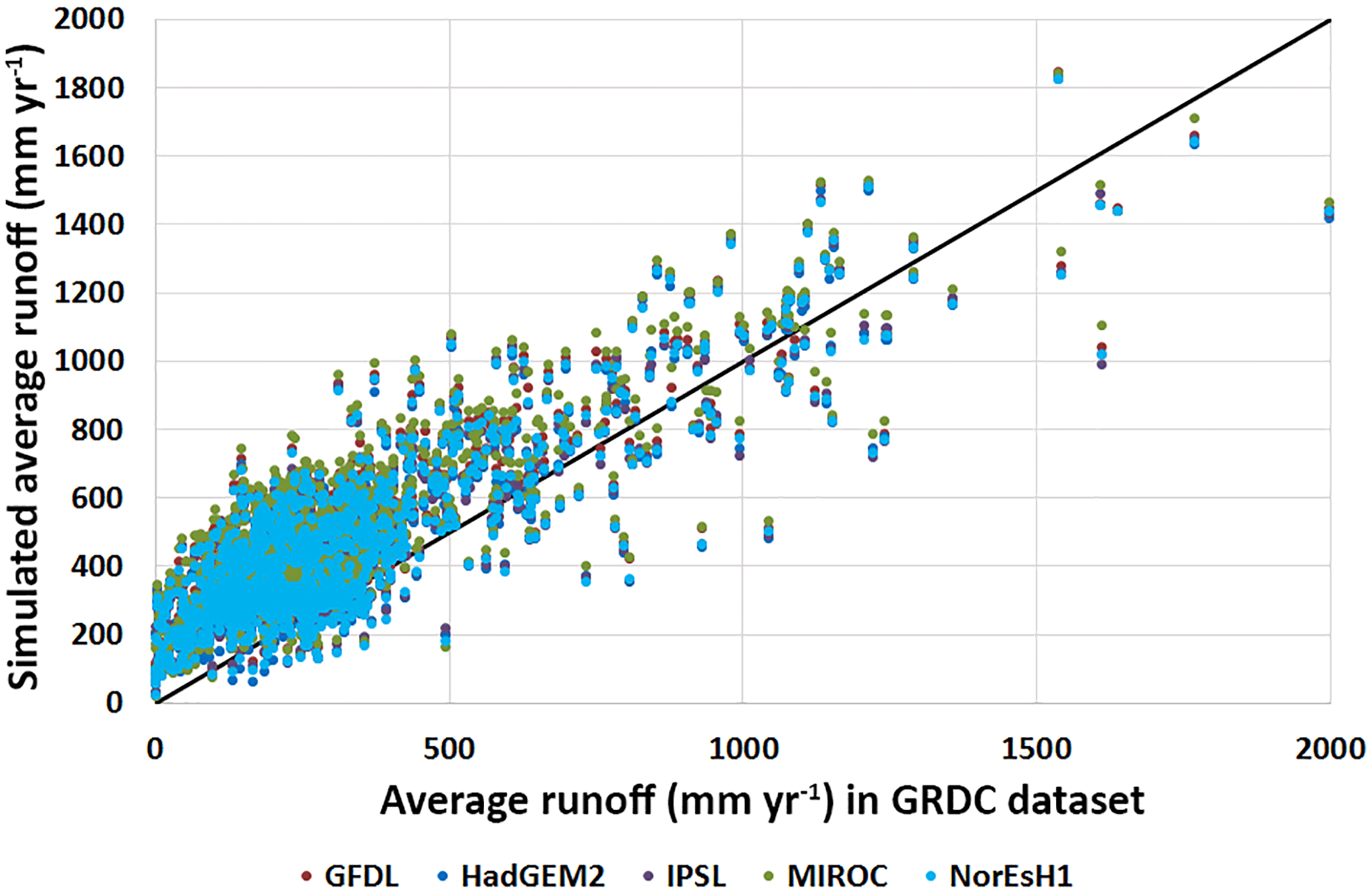
Figure 2Comparison of GRDC average runoff with simulated average runoff in subbasins according to PCR-GLOBWB model forced in the control period (1960–1999) with the five climate models.
Water availability values were routed through the river network producing the map shown in Fig. 3. The map shows the projected changes of water availability along the course of the main European rivers for the long term period under emission scenario RCP4.5 compared to the control period for the GFDL climate forcing. The projected changes with respect to current conditions are obtained through the comparison of the control and the climate change situation with an expression similar to Eq. (1). The results are patchier than in the case of runoff, due to the distortion introduced by the irregular distribution of reservoir storage and the changes in flow regime, which changes not only in mean but also in variability. Water availability may be more directly affected by changes in inter-annual or seasonal variability than by changes in mean annual runoff, especially if reservoir storage is small or inexistent.
We estimate the risk of water scarcity from changes in runoff and changes in water availability. The inherent assumption is that in countries under risk of water scarcity there is currently an approximate equilibrium between water availability and water demand, since water availability has been obtained through the progressive development of infrastructure to balance estimated demand. Assuming that we start from an equilibrium condition, we hypothesize that risk of water scarcity is linked to potential reduction of runoff and water availability.
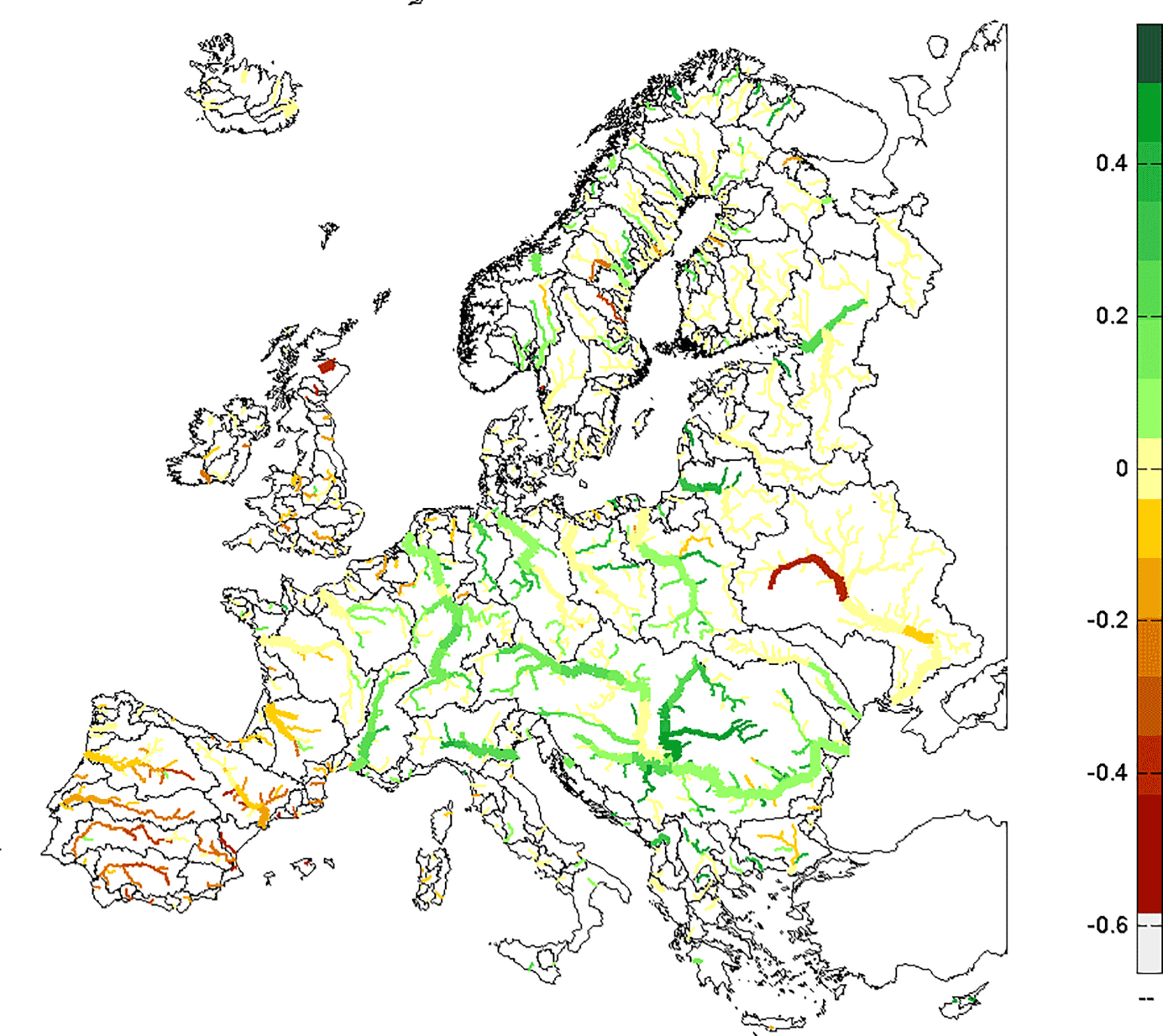
Figure 3Relative changes of water availability in the long term period (2060–2099) with respect to the control period (1960–1999) under emission scenario RCP4.5 according to PCR-GLOBWB model forced with GFDL climate data.
3.1 Rationale for the analysis
The basis for the analysis is the scatter plot of changes in runoff (ΔR) versus changes in water availability (ΔWA) for all basins under analysis. An example is shown in Fig. 4, corresponding to changes in the long term period (2060–2099) with respect to the control period (1960–1999) under emission scenario RCP4.5 with GFDL forcing. This figure shows results for subbasins (lighter colors) and global basins draining to the sea (darker colors).
Four quadrants are identified in Fig. 4. In the first quadrant, both runoff and water availability changes are positive (ΔR>0 and ΔWa>0). In this case, there is little risk of water scarcity unless water demands grow more than water availability. In the second quadrant, changes of water availability are positive, but changes in runoff are negative (ΔR<0 and ΔWA>0). As discussed above, this can happen for certain changes in the flow regime. In this case there is a mild risk of water scarcity because the reduction of runoff might stress the water supply system. In the third quadrant, changes in water availability are negative although changes in runoff are positive (ΔR>0 and ΔWA<0). This corresponds to a significant risk of water scarcity. Finally, in the fourth quadrant, both water availability and runoff experience negative changes (ΔR<0 and ΔWA<0). This is the condition with greatest risk of water scarcity.
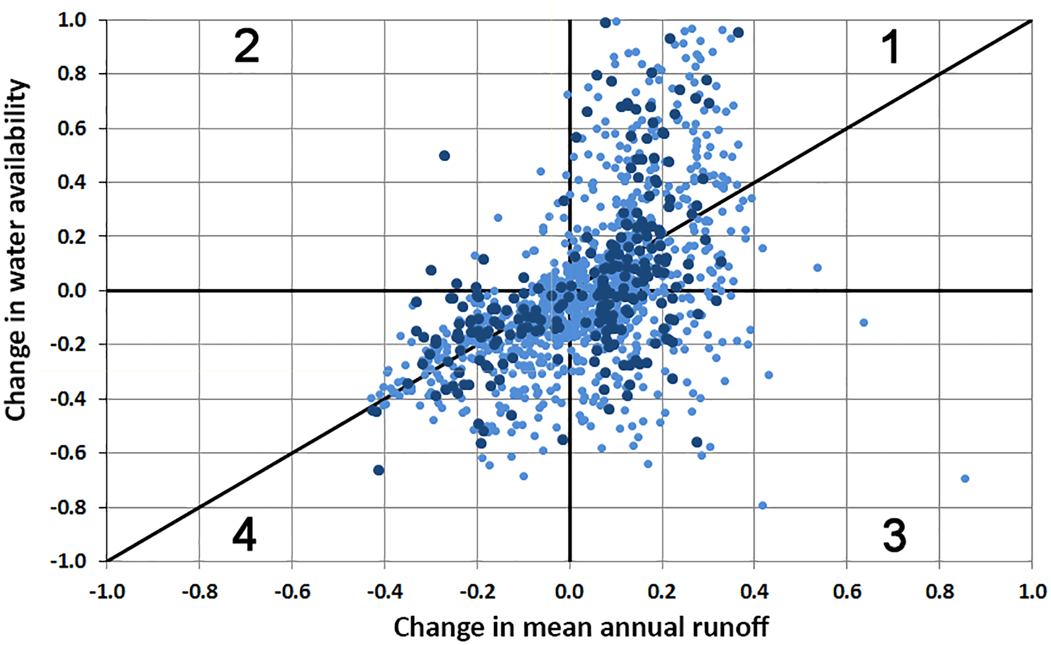
Figure 4Scatter plot of relative changes in runoff and water availability in the long term period (2060–2099) with respect to the control period (1960–1999) under emission scenario RCP4.5 according to PCR-GLOBWB model forced with GFDL climate data. Light dots correspond to individual subbasins and darker dots correspond to global basins draining to the sea.
The above analysis can be applied to an individual simulation. If there is an ensemble of realizations corresponding to different models, the different results obtained should be summarized in one single index.
Table 2Computation of the water scarcity risk index for emission scenario RCP4.5 in the long term (2060–2099) period.
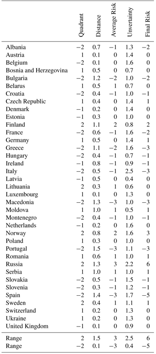
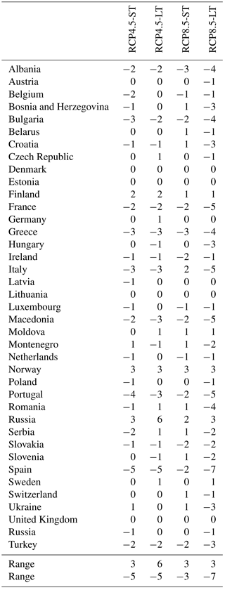
Table 3Country estimates of water scarcity risk index for emission scenarios RCP4.5 and RCP8.5 in the short term (ST: 2020–2059) and long term (LT: 2060–2099) periods.
3.2 Water scarcity index
We propose a water scarcity risk index based on two factors: the risk corresponding to average conditions IAVE and an uncertainty factor IUN.
The risk corresponding to average conditions IAVE is obtained from the position of the point representing the average of the simulations performed in the scatter plot of changes in runoff and changes in water availability. Its value is the product of two factors, following Eq. (2):
Where IQUAD is a risk factor depending on the quadrant and IDIST is a risk factor depending on the distance to the origin of coordinates. IQUAD is given relative values depending on the position of the point representing the average values of the simulations. The basic idea is that a decrease in water availability is a positive risk and an increase a negative risk. If the reduction of availability occurs in conjunction with a reduction of runoff, the risk is considered to be worse than if runoff is increasing. A similar criterion was applied to the increase in water availability. For points in the first quadrant (ΔR>0 and ΔWA>0) IQUAD takes a value of 2, for points in the second quadrant (ΔR<0 and ΔWA>0) it takes a value of 1, for points in the third quadrant (ΔR>0 and ΔWA<0) it takes a value of −1 and for points in the fourth quadrant (ΔR<0 and ΔWA<0) it takes a value of −2.
The second factor, IDIST, is obtained through the expression presented on Eq. (3):
Where w is a weighting factor that in our case is set to 5. This value was assigned to obtain a range of IAVE that would allow for a useful classification of countries according to their risk. IDIST represents the square of the distance from the origin of coordinates to the point representing the average of the simulations performed in the scatter plot of changes in runoff and changes in water availability.
The uncertainty factor IUN is obtained from the comparison of all simulations performed in the ensemble. This factor will be high if all realizations provide similar results, reinforcing the average result, and will be low if the realizations disagree, weakening the average result. This factor is obtained from the sum of the distances of the points representing individual realizations to the point representing the average result. Its expression is shown in Eq. (4):
Where n is the number of realizations and ΔRi and ΔWAi are the changes of runoff and water availability corresponding to realization i.
The water scarcity index described in the previous section was applied using countries as the spatial units of analysis. Country averaging is presented first, and then the procedure to obtain the water scarcity index is described.
4.1 Country averages
Country averaging introduces some difficulty in the analysis, since several countries may use water that is generated in upstream countries. The solution adopted was to consider locally available water first and add the possibility of using external water (coming from upstream cases) in certain countries.
The averaging was performed in two steps. In a first step, a dataset of country averages was produced for the runoff and incremental water availability variables for each of the hypotheses analyzed (model, emission scenario and time horizon). For example, if we consider RCP4.5 and time horizon 2020–2059, the country averages obtained for the changes of runoff and water availability variables are presented in Table 1. In the second step, significant water flows across boundaries were accounted by increasing water availability of downstream countries accordingly.
The results in terms of water availability do not always follow the pattern of runoff. Water availability is the result not only of mean annual runoff, but also of storage and variability. Climate scenarios imply changes in streamflow variability that affect water availability. Furthermore, the approach is clearly oversimplified in terms of spatial resolution and analytical methodology and has important limitations.
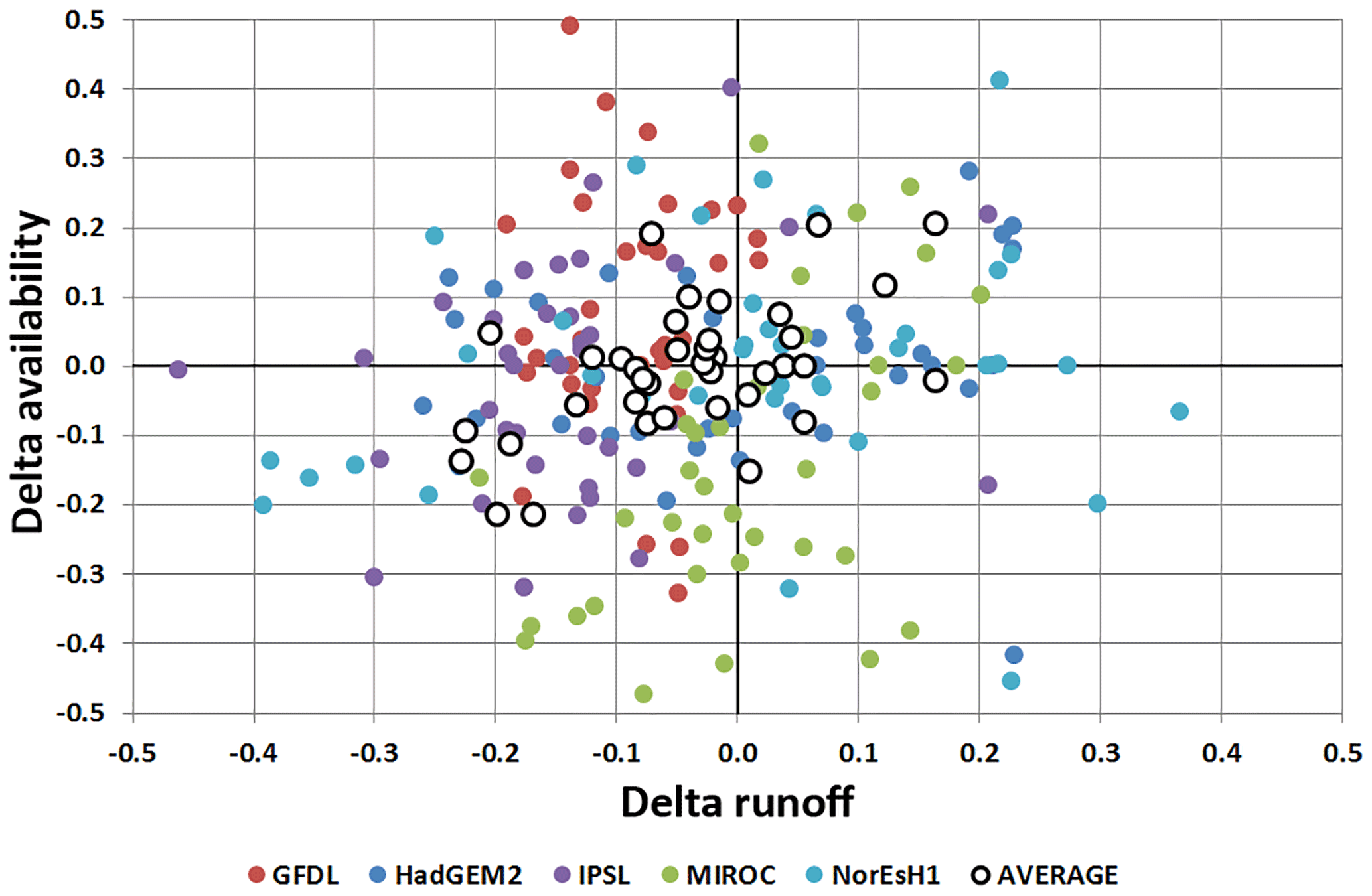
Figure 5Country estimates of changes in average runoff and surface water availability in the long term period (2060–2099) with respect to the control period (1960–1999) under emission scenario RCP4.5. Results show the five GCM forcing models considered and the average value.
The results presented in Table 1 are also shown graphically in Fig. 5, where the scatter plot of changes in runoff versus changes in water availability is presented at the country level. Individual model simulations are presented as coloured dots, while average values are presented as large white dots. Figure 6 presents examples of four individual countries, one in each of the four quadrants: Finland (first quadrant), Czech Republic (second quadrant), Netherlands (third quadrant) and Spain (fourth quadrant).
4.2 Index computations
The water scarcity indices were computed for all countries following the methodology described above. The detailed computation is shown in Table 2 for the emission scenario RCP4.5 and time horizon 2060–2099.
The final water scarcity risk index ranges from 6 to −5. The country with largest water scarcity risk is Spain (−5), followed by Portugal, Italy, Greece and Macedonia, all with a risk index of −3. These are all Southern European countries that are already exposed to water scarcity to some extent. There are more countries in the fourth quadrant, but with less risk of water scarcity, like France, Albania or Bulgaria. These countries are exposed to a reduction of both runoff and water availability, but the intensity of the reduction is comparatively smaller.
The final results obtained for the two emission scenarios (RCP4.5 and RCP8.5) and time periods (short term and long term) are presented in Table 3. The countries at larger risk are (in this order) Spain, Portugal, Macedonia, Greece, Bulgaria, Albania, France and Italy. All these countries show consistently negative values of the water scarcity index in the four scenarios analysed. They are mostly Mediterranean countries already exposed to significant water scarcity problems. Projections for them are negative, which means that significant adaptation measures are unavoidable.
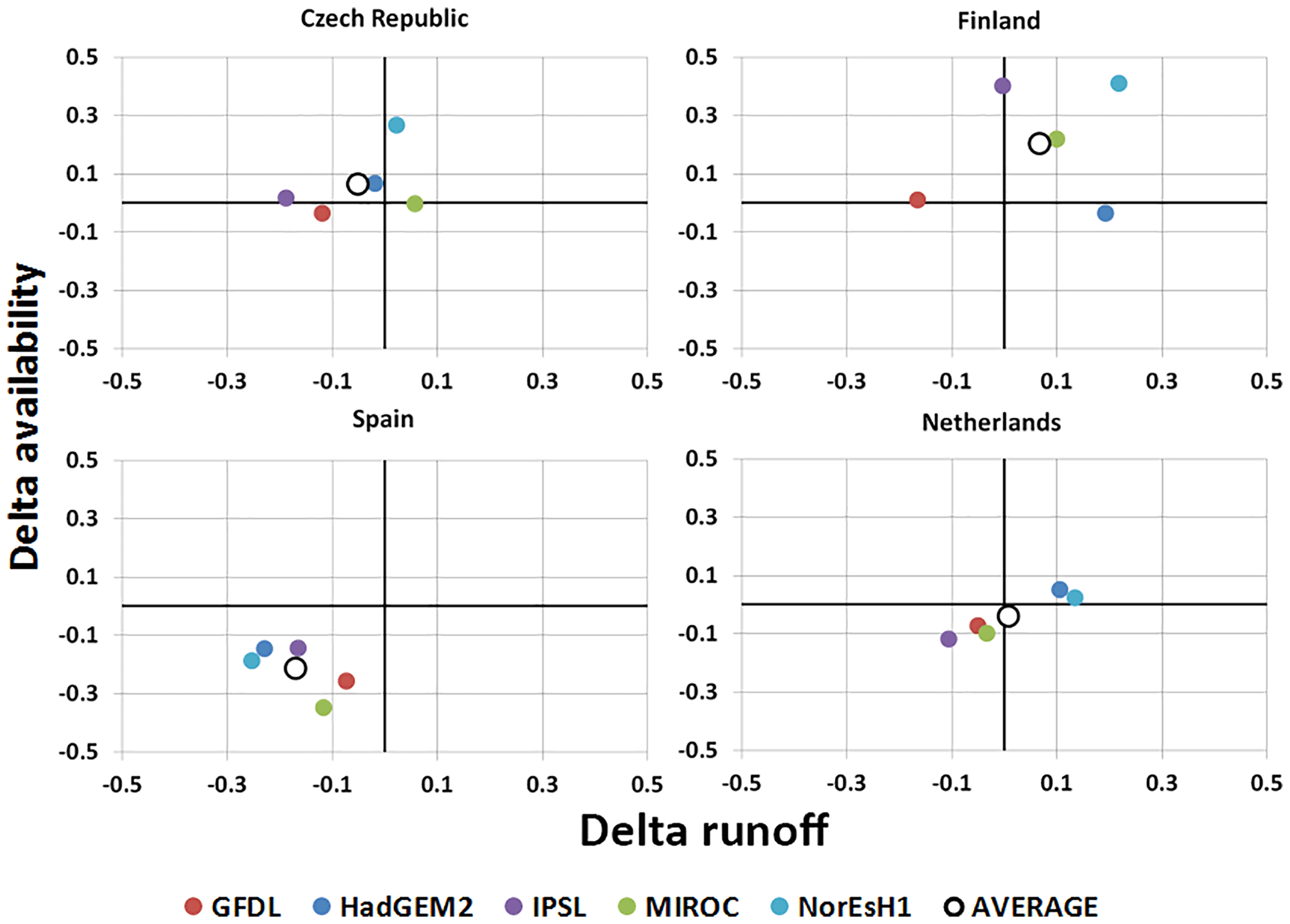
Figure 6Changes in annual runoff versus water availability for the model ensemble average (circles) and the individual GCMs (coloured dots) for RCP4.5 long term.
There are countries, like Slovakia, Belgium, Ireland, Croatia, Luxembourg, Romania, Netherlands, Hungary and Bosnia, with mild risk. Northern Arctic countries, like Sweden, Finland and Norway, show a robust however mild increase in water availability.
A regional assessment of water scarcity under climate change has been presented for Europe. The assessment is based on the water scarcity index, which is computed from the simulation results of changes in runoff and changes in water availability. The index summarizes the results obtained with several realizations under a certain emission scenario. It is based on two factors, one accounting for the average results and other accounting for the associated uncertainty.
The application of the water scarcity index to Europe provided a comparative picture of the exposure to risk of water scarcity induced by climate change in the countries of Europe. Countries at larger risk are those located in Southern Europe, particularly in the South East and in the South West.
Basic data for this work were obtained from publicly accessible databases. Topographic data were downloaded from the GTOPO HYDRO1k dataset, accessible in USGS Earth Explorer (https://earthexplorer.usgs.gov/), Entity ID: Entity ID:GT30H1KEU. Runoff data from the ISIMIP project were downloaded from the PIK node of the Earth System Grid Federation (ESGF) (https://esg.pik-potsdam.de/search/isimip-ft/), selecting Impact Model “PCR-GLOBWB”, Variable “Total Runoff” and Social Forcing “nosoc” (naturalized flows). Reservoir data were obtained from the ICOLD World Register of Dams (http://www.icold-cigb.net/GB/world_register/world_register_of_dams.asp), which is licensed for a fee.
The authors declare that they have no conflict of interest.
This article is part of the special issue “Innovative water resources management – understanding and balancing interactions between humankind and nature”. It is a result of the 8th International Water Resources Management Conference of ICWRS, Beijing, China, 13–15 June 2018.
We acknowledge the financial support of the European Commission BASE project (grant agreement no.: ENV-308337) of the 7th Framework Programme and the ADAPTA project, funded by Universidad Politecnica de Madrid.
We acknowledge the World Climate Research Programme's Working Group on
Regional Climate, and the Working Group on Coupled Modelling, former
coordinating body of CORDEX and responsible panel for CMIP5. We also thank
the climate modelling groups of models PCR-GLOBWB, GFDL-ESM2NM, HadGEM2-ES,
IPSL-CM5A-LR, MIROC-ESM-CHEM and NorESM1-M for producing and making
available their model output.
Edited by: Dingzhi Peng
Reviewed by: Hua Chen and one anonymous referee
Alcamo, J., Henrichs, T., and Rosch, T.: World Water in 2025: Global modeling and scenario analysis for the World Commission on Water for the 21st Century, Kassel World Water Series Report No. 2, CESR, Germany: University of Kassel, 1–49, 2000.
Alcamo, J., Döll, P., Henrichs, T., Kaspar, F., Lehner, B., Rösch, T., and Siebert, S.: Global estimates of water withdrawals and availability under current and future “business-as-usual” conditions, Hydrol. Sci., 48, 339–348, 2003a.
Alcamo, J., Döll, P., Henrichs, T., Kaspar, F., Lehner, B., Rösch, T., and Siebert, S.: Development and testing of the WaterGAP 2 global model of water use and availability, Hydrol. Sci., 48, 317–337, 2003b.
Alcamo, J., Floerke, M., and Maerker, M.: Future long-term changes in global water resources driven by socio-economic and climatic changes, Hydrol. Sci., 52, 247–275, 2007.
Arnell, N. W.: The Effect of Climate Change on Hydrological Regimes in Europe, Global Environ. Change, 9, 5–23,1999.
Arnell, N. W.: Climate change and global water resources: SRES emissions and socio-economic scenarios, Global Environ. Change, 14, 31–52, 2004.
Döll, P.: Impact of climate change and variability on irrigation requirements: A global perspective, Clim. Change, 54, 269–293, 2002.
EROS, USGS: HYDRO1k Elevation Derivative Database, Tech. rept., U.S. Geological Survey Center for Earth Resources Observation and Science (EROS), available at: https://lta.cr.usgs.gov/HYDRO1K, last access: 12 March 2018.
Fekete, B. M., Vörösmarty, C. J., and Grabs, W.: High-resolution fields of global runoff combining observed river discharge and simulated water balances, Global Biogeochem. Cy., 16, 1–6, 2002.
Fowler, H. J., Blenkinsop, S., and Tebaldi, C.: Linking climate change modelling to impacts studies: recent advances in downscaling techniques for hydrological modeling, Int. J. Climatol., 27, 1547–1578, 2007.
Fronzek, S. and Carter, T. R.: Assessing uncertainties in climate change impacts on resource potential for Europe based on projections from RCMs and GCMs, Clim. Change, 81, 357–371, 2007.
Garrote, L., Granados, A., and Iglesias, A.: Assessing Water Availability in Europe: a Comparative Study. Proceedings of the EWRA 2015 World Congress – Water Resources Management in a Changing World: Challenges and Opportunities, Istanbul, Turkey, 2015a.
Garrote, L., Iglesias, A., Granados, A., Mediero, L., and Martin-Carrasco, F.: Quantitative Assessment of Climate Change Vulnerability of Irrigation Demands in Mediterranean Europe, Water Resour. Manage., 29, 325–338, 2015b.
Gleick, P.: Global Freshwater Resources: Soft-Path Solutions for the 21st Century, Science, 302, 1524–1528, 2003.
ICOLD: World Register of Dams, International Commission on Large Dams, available at: http://www.icold-cigb.net/GB/world_register/world_register_of_dams.asp (last access: 14 September 2012), 2004.
IPCC: Chapter 3 of Climate Change 2014: Impacts, Adaptation and Vulnerability, Part A: Global and Sectoral Aspects, edited by: Field, C. B. and Barros, V. R., Cambridge University Press, 2014.
Sperna Weiland, F. C., van Beek, L. P. H., Weerts, A. H., and Bierkens, M. F. P.: Extracting information from an ensemble of GCMs to reliably assess future global runoff change, J. Hydrol., 412–413, 66–75, 2012.
van Beek, L. P. H. and Bierkens, M. F. P.: The Global Hydrological Model PCR-GLOBWB: Conceptualization, Parameterization and Verification Utrecht University, Faculty of Earth Sciences, Department of Physical Geography, Utrecht, The Netherlands, 2009.
Warszawski, L., Frieler, K., Huber, V., Piontek, F., Serdeczny, O., and Schewe, J.: The Inter-Sectoral Impact Model Intercomparison Project (ISI–MIP): Project framework, P. Natl. Acad. Sci. USA, 111, 3228–3232, 2014.
Wisser, D., Frolking, S., Douglas, E. M., Fekete, B. M., Vörösmarty, C. J., and Schumann, A. H.: Global irrigation water demand: Variability and uncertainties arising from agricultural and climate data sets, Geophys. Res. Lett., 34, L24408, https://doi.org/10.1029/2008GL035296, 2008.