the Creative Commons Attribution 4.0 License.
the Creative Commons Attribution 4.0 License.
 | 22 Apr 2020
Parameter estimation of a multiple aquifer-aquitard system from a single extensometer record: Las Vegas, Nevada, USA
Thomas J. Burbey
The purpose of this investigation is to develop a semi-analytical procedure for quantifying aquifer and aquitard properties from a single extensometer record in lieu of the time-consuming development of more complex numerical models to quantify and constrain these parameter values. Despite a limited 12-year record and the fact that water levels both decline and increase on an annual basis, estimates of both aquifer and aquitard parameters have been reasonably estimated at the Lorenzi extensometer site in Las Vegas Valley, Nevada when compared to the estimates developed numerically. The key factors that allow for accurate estimates of elastic and inelastic skeletal specific storage and hydraulic conductivity of the aquitards and elastic specific storage and hydraulic conductivity of the intervening aquifers is the presence of pumping cycles at multiple frequencies, and measured heads at all the aquifer units covered in the extensometer record and the inherent assumption that the aquitards have identical hydrologic characteristics and are homogeneous and isotropic. This latter assumption is also a usual limitation in numerical modelling of these settings because of the complex temporal head relationships occurring within the aquitards that are rarely, if ever, measured.


Extensometers have some distinct advantages over the satellite-based methods such as GPS and InSAR. Firstly, if designed properly, they can accurately measure compaction at the sub-millimetre or even to a few 10's of microns. Secondly, the data can be continuous so even if pumping occurs at diurnal frequencies, it is possible for the extensometer to record possible compaction from these high frequency pumping events. Thirdly, in many localities we have a much longer historical record with extensometers than we do with satellite data. Extensometer data have been available at some sites since the 1960s, when subsidence rates were much higher due to the fact that subsidence was not as yet well known as a consequence to excessive groundwater pumping. Fourthly, extensometers measure the compaction over the depth of the extensometer pipe, typically within the zone of active pumping (which is how they tend to be designed) so that tectonic and eustatic changes are not part of the deformation record. They are also not subject to topographic effects that often plague InSAR processing and can interfere with signal coherence. The two biggest disadvantages to the implementation of extensometers is the cost and the fact that they are point measurements. As such, it is uncommon for more than a few extensometers to exist within an entire aquifer system or basin.
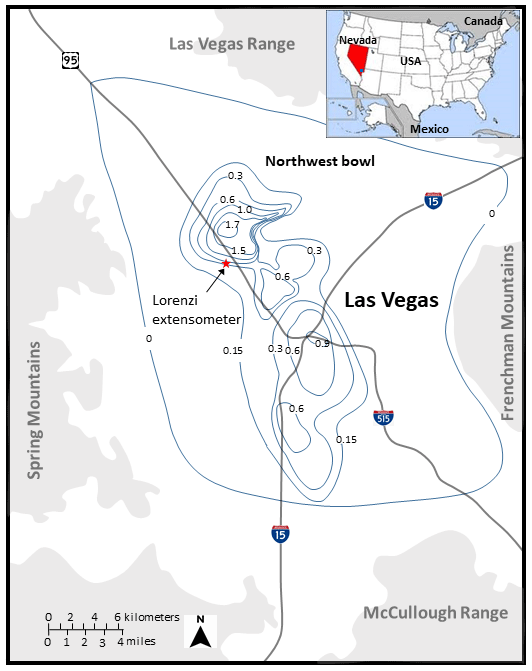
Figure 1Map of Las Vegas Valley showing the location of the Lorenzi extensometer site and estimated and measured land subsidence for the period 1963–1990 adapted from Bell et al. (2002).
Extensometer data, when coupled with continuous time-series water-level data in the aquifers through which the extensometer penetrates, can yield important aquifer system hydrologic properties (Epstein, 1987), particularly when cyclical pumping patterns occur at multiple frequencies. In this analysis, water-level data responding to multiple-frequency pumping patterns are used along with compaction data from a single extensometer record extending through a multiple aquifer/aquitard system at the Lorenzi site in Las Vegas, Nevada. The aim is to estimate important hydraulic parameters including the specific storage and hydraulic conductivity of the aquifers, and the elastic and inelastic specific storage and hydraulic conductivity of the aquitards.
Las Vegas Valley (Fig. 1) represents an extensional structural basin filled with more than 1500 m of alluvial deposits that have produced a complex and heterogeneous sequence of aquifers and aquitards of varying thickness and compressibility. A near-surface aquifer overlies a more extensive principal aquifer system from which domestic water originates in the valley. The principal aquifer system contains various confining layers that contribute to land subsidence. Pumping has occurred in the valley for approximately 100 years causing as much as 90 m of water-level decline (Burbey, 1995) and nearly 2 m of compaction in the northwest subsidence bowl since 1963 (Bell et al., 2002). The principal aquifer system contains three confining layers and three aquifers, referred to here as the shallow, middle, and deep confining layers and aquifers, respectively. The aquifers are composed largely of sands and gravels with minor thin layers of silts and clays, while the aquitard units are composed almost entirely of clays and silts. Drilling logs from the extensometer borehole (244 m total depth) and geophysical surveys have defined the depths and thicknesses of the aquifer and aquitard units within the larger principal aquifer system of the basin (Pavelko, 2000). Hourly water-level data from each of the three aquifers along with hourly compaction data were collected at the extensometer site from November 1994 to December 2007. The Lorenzi extensometer site is located within 3200 m of approximately 14 municipal pumping wells that pump at different diurnal and seasonal rates. Figure 2 shows the entire available water level and compaction record of the Lorenzi site. Fluctuations in diurnal water levels are not evident at the scale of Fig. 2. These daytime to-night-time water-level fluctuations are attributed to differences in daily pumping of 5400 m3 in the period of evaluation.
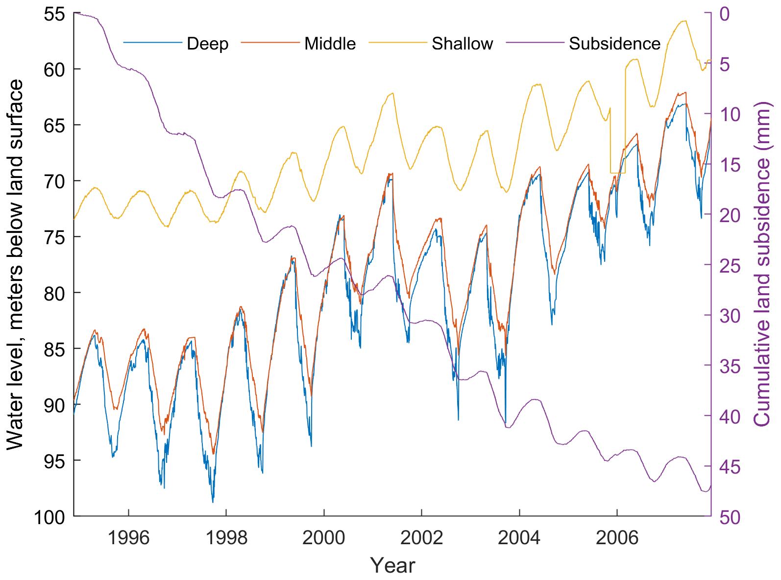
Figure 2Mean daily record of the compaction and water level records for the shallow, middle and deep aquifers at the Lorenzi extensometer site for the entire measured record, 1995–2007.
The methodology used here is a three-step process in which the first step involves the evaluation of aquifer elastic storage and horizontal hydraulic conductivity using the Theis equation by taking advantage of the diurnal pumping signals that reflect the aquifer conditions only. The second step involves the evaluation of aquitard elastic skeletal storage and vertical hydraulic conductivity of the aquitard units. The assumption here is that all the aquitard units have the same hydraulic properties. The long-term inelastic signal is removed from the record using a low-pass filter. Seasonal periodic pumping is used as this frequency of pumping elastically deforms a portion of aquitards on a yearly basis. The portion of aquitard thickness undergoing elastic deformation is determined in this process. The third step involves the evaluation of aquitard inelastic storage, which is based on the known pumping history and the nature of the inelastic deformation time-series. In this approach, a time constant for the aquitard is approximated based on aquitard thickness, the calculated hydraulic conductivity (from step 2) and the nature of the inelastic compression.
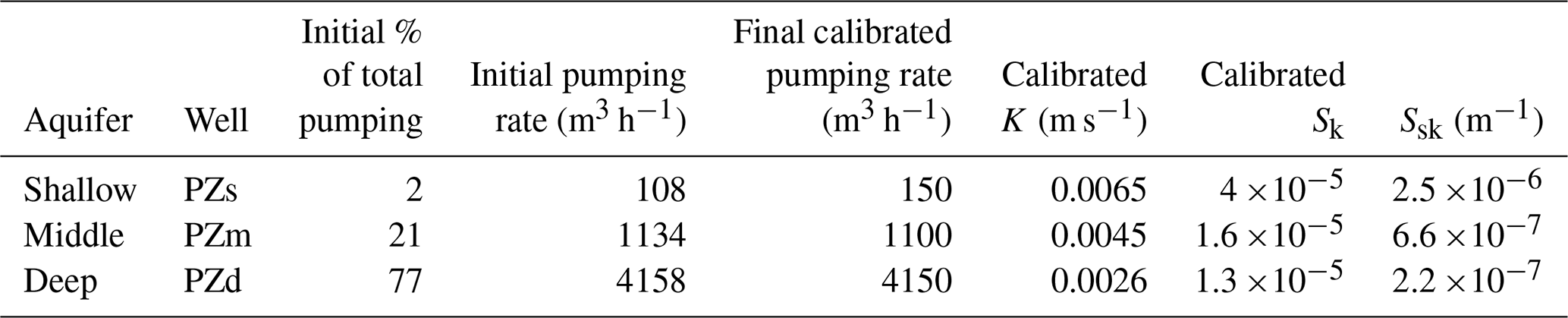
Table 1Calibrated hydraulic conductivity and storage parameters for the shallow, middle and deep aquifers using the Theis equation (Eq. 1) for cyclical daily pumping.
The first step in analysing the aquifer system of the Lorenzi extensometer site is to attempt to quantify the aquifer properties by using daily periodic water levels attributed to diurnal fluctuations caused by daily pumping cycles, which isolates the aquifer response and is too quick to induce leakage and subsequently compaction of the intervening confining units. For this analysis a 5-day period in June 1998 is chosen where pumping and recovery periods are known as well as the pumping rates (Pavelko, 2000). Under diurnal pumping cycles the aquifers behave as confined units, which can be readily analysed using the Jacob formulation of the Theis equation and implementing periodicity (Eq. 1):
where s is the drawdown, Q is the pumping rate and the subscript (k) refers to the aquifer (shallow, middle or deep), K is the hydraulic conductivity, b is the aquifer thickness, r is the distance from the pumping well to the observation wells, S is the storage coefficient, t is the total time (over all cycles of pumping) and t1 is the time since pumping stopped. Pumping is apportioned to each aquifer based on the cumulative relative head change over the range of the five cycles for the aquifer compared to the total head change across all three aquifers (expressed as a percentage). This approach yields the total pumping fractions of 0.02, 0.21 and 0.77 for the upper, middle and lower aquifers, respectively. Table 1 (columns 3–5) shows the initial and calibrated pumping rates for each aquifer based on these percentages. Parameters are optimized by minimizing an objective function representing the sum of the squared residuals of drawdown for the 5 cycles of pumping and recovery for each aquifer.

Figure 3(a) long term compaction (blue) with trend line (orange), (b) long-term compaction trend removed to reveal annual compaction pattern over period of record, and (c) annual compaction (blue) with sine wave fit (orange) showing mean frequency and amplitude of annual elastic compaction due to persistent seasonal pumping patterns.
The second step is to evaluate the elastic aquitard parameters from the seasonal periodic pumping patterns associated with high summer pumping demand and winter recovery, which is enhanced with a known quantity of artificial recharge (injection). Because no water-level data are available from within any of the aquitards and because only one composite compaction record is available, it must be assumed that each of the three aquitards (thicknesses are 78, 34 and 32 m, respectively) exhibit the same behavior and thus have the same parameter values of vertical hydraulic conductivity and elastic storage. Furthermore, it is hypothesized that the seasonal elastic response of the total compaction is attributed largely to the confining units and is associated with the seasonal head changes in the aquifers. From the seasonal pumping cycle, a cross-spectral analysis over the 12-year record showed that no significant lag exists between what is deemed as the elastic aquitard response and the seasonal water-level record.
To isolate the seasonal elastic response of the system, a low-pass filter is used to remove the long-term decadal trend (inelastic component) of system compaction (Fig. 3) and then to fit a periodic sine function to the seasonal elastic response. The mean seasonal elastic recovery can then be readily calculated from the mean fitted periodic curve and is 2.7 mm. Next, we can identify the seasonal compaction contribution of each aquifer from the total seasonal compaction record through the following equation:
where Δb is the compaction in an aquifer i (i=1–3, n=3), S is the storage coefficient for the aquifer evaluated from the Theis equation (Table 1), and Δh is the seasonal head change shown for each aquifer (i). By deconvolving the total head record for each aquifer and isolating the seasonal head change using a low-pass filter, the longer decadal trend is removed from the record. The head change is then fitted to a mean sine function, which represents the mean seasonal head amplitude over the period of record as shown in Fig. 4 (only deep aquifer shown). The middle plot (labeled b) of the figure leaves only the seasonal changes for each year while the lower plot shows the sine function fit and represents the frequency and mean amplitude for the entire period of record. From this analysis, the total seasonal head change for the shallow, middle, and deep aquifers is 4.70, 8.04 and 10.23 m, respectively. Multiplying these head changes by the aquifer storage coefficient according to Eq. (2), yields aquifer compactions for the shallow, middle, and deep aquifers of 0.19, 0.13 and 0.13 mm, respectively. The sum produces a cumulative compaction assigned to the three aquifers of 0.45 mm. This outcome reveals that 26 % of the total seasonal compaction is attributed to the aquifers. Therefore, the remaining 74 % of the seasonal compaction, or 2.25 mm, must be coming from the three aquitards. Using the aquifer relative head changes results in 20 %, 35 % and 45 % of the total compaction originating from the upper, middle and lower aquitards, respectively. This translates to a total compaction assigned to each of the three aquitards as 0.45, 0.79, and 1.01 mm, respectively.
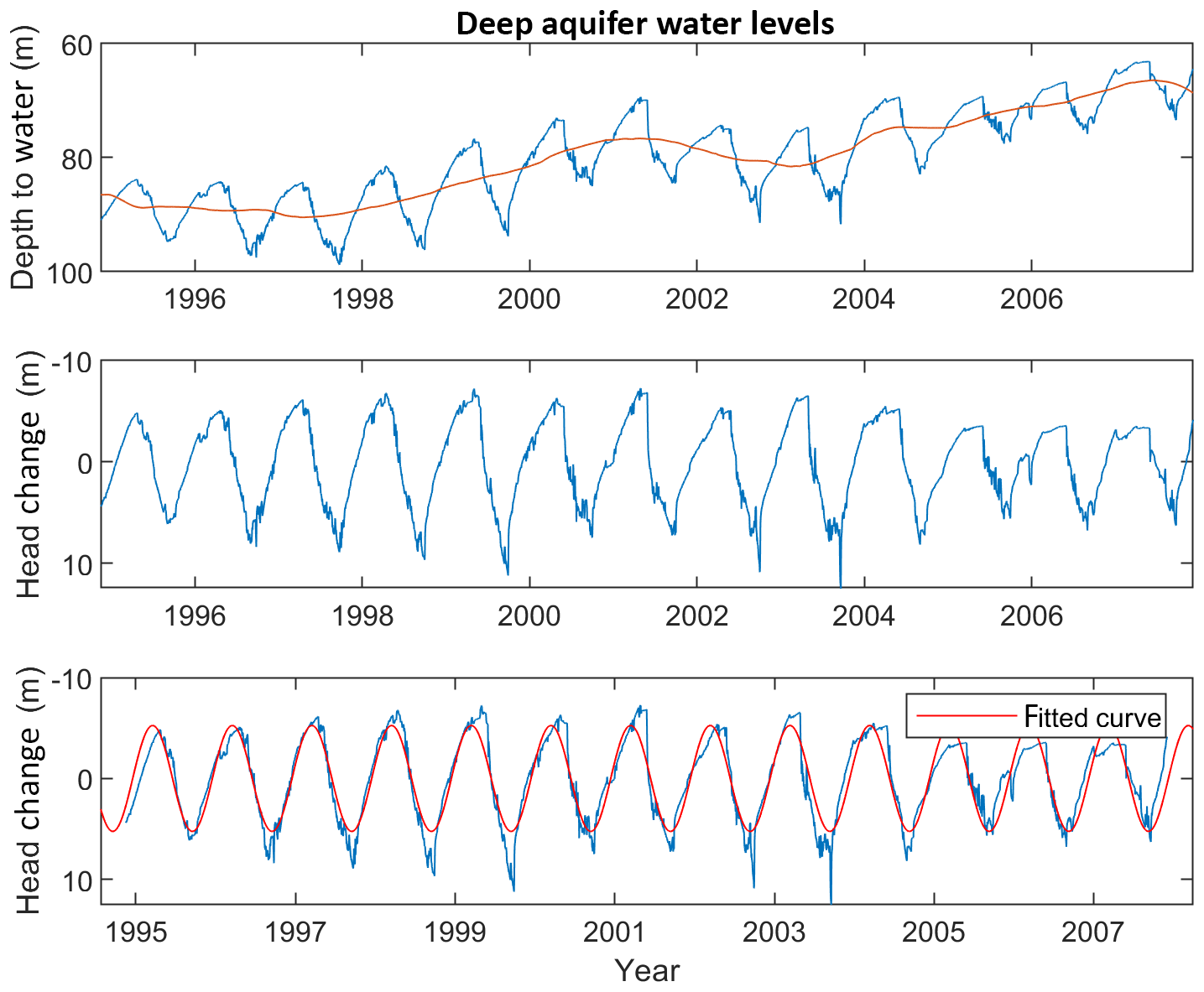
Figure 4(a) Long-term deep piezometer record (blue) with trend line (orange), (b) seasonal water levels with trend removed and (c) seasonal water levels (blue) with fitted sine function (orange) revealing mean frequency and amplitude of water levels in the shallow aquifer.
For a singly draining unit (aquifer head decline causes an elastic response to one side of the aquitard) the time constant is defined as:
where the primes indicate the variables pertain to the aquitard and b′ is the length of the drainage path, is the vertical hydraulic conductivity of the aquitard and is the aquitard skeletal specific storage. In this analysis we take a reverse approach and assume the time constant to be equal to the seasonal pumping period of 182 days. This effectually produces the effective thickness of the aquitard that undergoes elastic deformation. We know that during this time period the aquitard acts elastically so the specific storage will represent the elastic component (). Under these conditions b′ refers to the thickness of the confining unit undergoing elastic deformation during the time of pumping. This thickness is independent of the magnitude of head change occurring within the unit. Figure 5 shows a plot of different elastic confining unit thicknesses for different values of elastic skeletal specific storage and vertical aquitard hydraulic conductivity. The shaded box shows the range of values obtained from the literature from eight different sites across the country where extensometer data were used to obtain aquitard parameter values either graphically (stress-strain diagrams), or numerically (one or two dimensional flow and compaction models) (Epstein, 1987; Hanson, 1989; Heywood, 2003; Pavelko, 2004; Pope and Burbey, 2004; Riley, 1969; Sneed and Galloway, 2000). The point within the box is the numerically calibrated values of these aquitard parameters from Pavelko (2004) for the Lorenzi site in Las Vegas. Based on these data, the elastic aquitard thickness undergoing seasonal response varies from 3 to 5 m with 4 m being the average and optimal value used in this analysis with 3 and 5 m representing the upper and lower range of reasonable thicknesses, respectively. This thickness represents the vertical extent into the aquitards directly adjacent to the aquifers that responds elastically to the seasonal head changes in the adjacent aquifers. The skeletal elastic storage coefficient can now be estimated by the simple relation, .
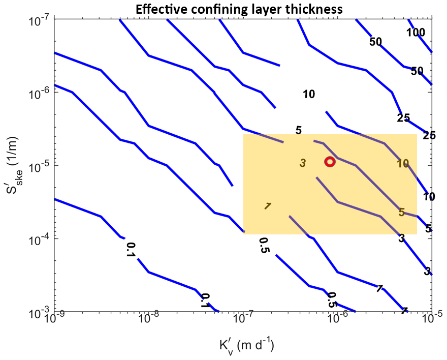
Figure 5Plot of aquitard thicknesses responsible for contributing to elastic compaction associated with seasonal head changes for a range of elastic skeletal specific storage values and hydraulic conductivity values of the confining units. The orange box represents the range of parameter values found in the literature for extensometer sites in the United States. The red circle represents the optimal values from the numerical analysis of Pavelko (2004).
Since we have assumed homogeneous conditions for the aquitards we can realistically only use a mean value for the skeletal specific storage. Furthermore, since we calculated the thickness of the compacting confining unit to be 8, 8, and 4 m, respectively surrounding the upper, middle and deep aquifers, the elastic skeletal specific storage can also be readily calculated. The mean optimal skeletal storage and skeletal specific storage values are calculated to be and m−1 respectively. Finally, using Eq. (3) to solve for the confining unit hydraulic conductivity yields an estimate of m d−1. These values are all within 10 % of those numerically calculated by Pavelko (2004).
Step three in the parameter estimation process involves estimation of the inelastic skeletal specific storage of the confining units. The difficulty in this estimation lies in the fact that the heads in the confining layers are not in equilibrium with the measured heads in the aquifers due to the slow release of water from these units, creating a hydrodynamic lag between the heads in the aquifer and the observed compaction. Because the heads in the first few years of the data set (Fig. 2) are decreasing and the heads in later years are recovering, the resulting heads in the confining units show a continual decline at their centers (expulsion of water), but show both declining and increasing heads in the portions of the aquitards nearest the aquifers (the elastic aquitard response).
The long-term trend (annual to decadal compaction) in compaction (Fig. 3) shows a significant change in slope that is associated with the slowing of drainage from the aquitards as the heads in the aquifers begin to recover. A linear annual trend can be found when plotting heads against compaction data with a high degree of correlation. However, the slope associated with such a trend does not reflect the inelastic specific storage of the confining units.
In this analysis, a semi-analytical approach is used to estimate . Since it's likely that compaction has been ongoing (no uplift) at this site since the inception of pumping in Las Vegas Valley, we set the time constant equal to the total time of pumping (and co mmencement of head declines), which is roughly 90 years. This value is reasonable for the thicknesses of the middle and lower confining units based on estimates from this and other systems (Epstein, 1987; Pavelko, 2004; Sneed and Galloway, 2000). Using Riley's (1969) expression for the time constant for doubly draining aquitards and rearranging to solve for the specific storage, which in this case now refers to the inelastic skeletal specific storage of the confining units
The thickness of each of the lower two aquitards is nearly identical so an average thickness of 33 m is used here. Different possible time constants for the average confining unit thickness of 33 m are calculated for a range of hydraulic conductivity and inelastic skeletal specific storage values of the confining units. Using 90 years as the time constant represents the minimum realistic time constant since compaction is still occurring (Fig. 2) in the inelastic range from the inception of pumping. Furthermore, since the water-level recoveries are clearly impacting the slope of the long-term compaction record, it is unlikely the time constant for these confining units is likely to exceed 200 years. Figure 3a shows that the compaction is asymptotically approaching zero temporal change, which implies that the dispersive flux from the aquitards is decreasing at the same rate as the rate of compaction (assuming constant parameter values for and ). This result at least qualitatively implies that the aquitard is approaching equilibrium with the heads in the aquifer. Even with a 110-year possible length for the time constant, this greatly narrows the possible range of viable values to a factor of only 2. The 90-year time constant yields a calculation of m−1, which is nearly identical to the value produced numerically by Pavelko (2004).
The goal of this investigation is to determine if a simplistic semi-analytical approach could be used to reasonably quantify the aquifer and aquitard parameters at a point site (extensometer) in lieu of having to build a more complex and time-consuming numerical model to estimate parameter values. With careful examination, extensometer data can provide more than just a continuous record of the total compaction history associated with the lowering of hydraulic heads within the measured zone of the extensometer pipe. This investigation reveals that important parameter values of the aquifer and aquitards including the hydraulic conductivities and elastic and inelastic specific storage can be reasonably quantified under the following conditions: (1) all hydrostratigraphic units important to the overall compaction record have been identified and their thicknesses established, (2) all the intervening aquifer hydraulic heads are measured over the length of the extensometer pipe, (3) cyclical pumping patterns are available for the length of the record and preferably at multiple temporal frequencies, and (4) a reasonable historic understanding of the length of the pumping history affecting the measured record.
The time series data used in this investigation will be available on the CUAHSI HydroShare web site and is available upon request to the author in the meantime.
The author declares that there is no conflict of interest.
This article is part of the special issue “TISOLS: the Tenth International Symposium On Land Subsidence – living with subsidence”. It is a result of the Tenth International Symposium on Land Subsidence, Delft, the Netherlands, 17–21 May 2021.
Bell, J. W., Amelung, F., Ramelli, A. R., and Blewitt, G.: Land subsidence in Las Vegas, Nevada, 1935–2000: New geodetic data show evolution, revised spatial patters, and reduced rates, Environ. Eng. Geosci., 8, 155–174, 2002.
Burbey, T. J.:Pumpage and water-level change in the principal aquifer of Las Vegas Valley, Nevada, 1980–90, U.S. Geological Survey Water-Resources Information Report no. 34, 224 pp., 1995.
Epstein, V. J.: Hydrologic and geologic factors affecting land subsidence near Eloy, Arizona, U.S. Geological Survey, Tucson, Arizona, 28 pp., 1987.
Hanson, R. T.: Aquifer-system compaction, Tucson Basin and Avra Valley, Arizona, Water-Resources Investigations Report 88-4172, U.S. Geological Survey, 69 pp., 1989.
Heywood, C. E.: Summary of extensometric measurements in El Paso, Texas, Water-Resources Investigations Report 03-4158, U.S. Geological Survey, 11 pp., 2003.
Pavelko, M. T.: Ground-water and aquifer-system-compaction data from the Lorenzi Site, Las Vegas, Nevada, 1994p-1999, U.S. Geological Survey Circular Open-File Report 00-362, 2000.
Pavelko, M. T.: Estimates of hydraulic properties from a one-dimensional numerical model of vertical aquifer-system deformation, Lorenzi Site, Las Vegas, Nevada, U.S. Geological Survey Water-Resources Investigations Report 03-4083, 35 pp., 2004.
Pope, J. P. and Burbey, T. J.: Multiple-aquifer characterization from single borehole extensometer records, Ground Water, 42, 45–58, 2004.
Riley, F. S.: Analysis of borehole extensometer data from central California, International Association of Hydrologic Sciences, Publication no. 89, 423–431, 1969.
Sneed, M. and Galloway, D. L.: Aquifer-system compaction and land subsidence: Measurements, analyses, and simulations–the Holly Site, Edwards Air Force Base, Antelope Valley, California, U.S. Geological Survey, Water-Resources Investigations Report 00-4015, 68 pp., 2000.